Mastering Pandas for Efficient Data Manipulation and Analysis

What is Pandas?

Pandas is a powerful library for data manipulation and analysis in Python. It provides data structures and functions to efficiently handle structured data, including tabular data such as spreadsheets and SQL tables.

Key Features of Pandas

Data Structures: Series (1D) and DataFrame (2D) for flexible data handling.
Data Manipulation: Merge, reshape, select, and clean data with ease.
Data Analysis: Descriptive statistics, data visualization, and time series analysis tools.
Integration: Seamless integration with NumPy, Matplotlib, and SciPy for enhanced functionality.

Why Use Pandas?

Efficiency: Designed to handle large datasets with ease.
Ease of Use: Intuitive syntax simplifies complex data tasks.
Community Support: Active community ensures extensive documentation and support.

Getting Started with Pandas

Install Pandas using pip:

pip install pandas

Import Pandas in your Python script:

import pandas as pd

Example: Creating a DataFrame


import pandas as pd

data = {
  'Name': ['Alice', 'Bob', 'Charlie'],
  'Age': [25, 30, 35],
  'City': ['New York', 'Los Angeles', 'Chicago']
}

df = pd.DataFrame(data)
print(df)

Output:


      0    Alice
      1    Bob
      2    Charlie
      dtype: object

Setting Up Your Environment for Pandas

Installing Pandas

pip install pandas

Setting Up a Virtual Environment


  # Create a virtual environment
  python -m venv myenv
  
  # Activate the virtual environment
  # On Windows
  myenv\Scripts\activate
  # On macOS/Linux
  source myenv/bin/activate
  
  # Install Pandas in the virtual environment
  pip install pandas

Choosing the Right IDE for Pandas Development

Jupyter Notebook: Ideal for interactive data analysis and visualization.
PyCharm: A powerful IDE with advanced features like code completion, debugging, and version control integration.
VS Code: A lightweight, highly customizable editor with extensions for Python development, including Jupyter support.

Setting Up Jupyter Notebook

pip install notebook

jupyter notebook

Understanding Data Structures in Pandas: Series and DataFrames

Introduction to Pandas Series

A Pandas Series is a one-dimensional array-like object that can hold data of any type (integers, strings, floating points, etc.).

Homogeneous Data: All elements in a Series are of the same data type.
Indexing: Each element is indexed, providing fast access to data.
Operations: Supports vectorized operations, making data manipulation efficient.


  import pandas as pd
  data = [10, 20, 30, 40]
  series = pd.Series(data)
  print(series)

Output:


  0    10
  1    20
  2    30
  3    40
  dtype: int64

Deep Dive into Pandas DataFrames

A Pandas DataFrame is a two-dimensional, size-mutable, and potentially heterogeneous tabular data structure with labeled axes (rows and columns).

Heterogeneous Data: Can hold different data types (integer, float, string, etc.) in different columns.
Labeled Axes: Both rows and columns have labels, making data manipulation intuitive.
Operations: Supports a wide range of operations such as filtering, grouping, and merging.


  import pandas as pd
  data = {
    'Name': ['Alice', 'Bob', 'Charlie'],
    'Age': [25, 30, 35],
    'City': ['New York', 'Los Angeles', 'Chicago']
  }
  df = pd.DataFrame(data)
  print(df)

Output:


      0    Alice, 25, New York
      1    Bob, 30, Los Angeles
      2    Charlie, 35, Chicago
      dtype: object

Additional Information

Operations on Series and DataFrames

Series Operations: Element-wise operations, apply functions, and methods like .sum(), .mean(), and .apply().
DataFrame Operations: Support for .groupby(), .merge(), .pivot(), and .join(), essential for data analysis and manipulation.

Use Cases

Series:
- Ideal for time series data
- Suitable for single columns of data
- Simple data manipulations
DataFrames:
- Suitable for complex data analysis
- Multi-dimensional data
- Operations involving multiple columns

Working with Data in Pandas: A Comprehensive Guide

Importing and Exporting Data with Pandas

Pandas provides robust functions to read and write data from various file formats, making it easy to import data into your DataFrame and export it for further use.

Reading Various File Formats

Reading CSV Files

CSV (Comma-Separated Values) files are one of the most common data formats. Pandas makes it straightforward to read CSV files into a DataFrame.


  import pandas as pd
  
  # Reading a CSV file
  df_csv = pd.read_csv('data.csv')
  print(df_csv.head())

Reading Excel Files

Excel files are widely used in data analysis. Pandas can read Excel files, including specific sheets.


  import pandas as pd
  
  # Reading an Excel file
  df_excel = pd.read_excel('data.xlsx', sheet_name='Sheet1')
  print(df_excel.head())

Reading JSON Files

JSON (JavaScript Object Notation) is a popular format for data exchange. Pandas can easily read JSON files into a DataFrame.


  import pandas as pd
  
  # Reading a JSON file
  df_json = pd.read_json('data.json')
  print(df_json.head())

Writing Data to Files

Pandas also makes it easy to export data from your DataFrame to various file formats.

Writing to CSV Files


  import pandas as pd
  
  # Writing to a CSV file
  df.to_csv('output.csv', index=False)

Writing to Excel Files


  import pandas as pd
  
  # Writing to an Excel file
  df.to_excel('output.xlsx', sheet_name='Sheet1', index=False)

Writing to JSON Files


  import pandas as pd
  
  # Writing to a JSON file
  df.to_json('output.json', orient='records')

Handling Different File Formats

CSV Files

Use pd.read_csv() and df.to_csv() for reading and writing CSV files. You can specify parameters like delimiter, header, and index.


  import pandas as pd
  
  # Reading a CSV file
  df = pd.read_csv('data.csv', delimiter=',', header=0, index_col=0)
  
  # Writing to a CSV file
  df.to_csv('output.csv', index=False)

Excel Files

Use pd.read_excel() and df.to_excel() for Excel files. You can specify the sheet name and other parameters.


  import pandas as pd
  
  # Reading an Excel file
  df = pd.read_excel('data.xlsx', sheet_name='Sheet1')
  
  # Writing to an Excel file
  df.to_excel('output.xlsx', sheet_name='Sheet1', index=False)

JSON Files

Use pd.read_json() and df.to_json() for JSON files. You can specify the orientation and other parameters.


  import pandas as pd
  
  # Reading a JSON file
  df = pd.read_json('data.json', orient='records')
  
  # Writing to a JSON file
  df.to_json('output.json', orient='records')

Common Operations

Filtering Data

Use methods like .loc[] and .iloc[] to filter data based on conditions.


  import pandas as pd
  
  # Create a sample DataFrame
  df = pd.DataFrame({
      'Name': ['Alice', 'Bob', 'Charlie'],
      'Age': [25, 30, 35]
  })
  
  # Filter data using .loc[]
  filtered_df = df.loc[df['Age'] > 30]
  print(filtered_df)

Grouping Data

Use .groupby() to group data and perform aggregate functions.


  import pandas as pd
  
  # Create a sample DataFrame
  df = pd.DataFrame({
      'Name': ['Alice', 'Bob', 'Charlie'],
      'Age': [25, 30, 35],
      'City': ['New York', 'Los Angeles', 'Chicago']
  })
  
  # Group data by City and calculate mean Age
  grouped_df = df.groupby('City')['Age'].mean()
  print(grouped_df)

Merging Data

Use .merge() to combine DataFrames based on common columns.


  import pandas as pd
  
  # Create two sample DataFrames
  df1 = pd.DataFrame({
      'Name': ['Alice', 'Bob', 'Charlie'],
      'Age': [25, 30, 35]
  })
  df2 = pd.DataFrame({
      'Name': ['Alice', 'Bob', 'Charlie'],
      'City': ['New York', 'Los Angeles', 'Chicago']
  })
  
  # Merge DataFrames on the 'Name' column
  merged_df = pd.merge(df1, df2, on='Name')
  print(merged_df)

Handling Different Data Sources

Databases

Pandas can connect to various databases using libraries like SQLAlchemy for SQL databases. This allows you to read from and write to databases directly.

Example: Reading from a SQL Database


  import pandas as pd
  from sqlalchemy import create_engine
  
  # Create an engine instance
  engine = create_engine('sqlite:///mydatabase.db')
  
  # Read data from a SQL table
  df_sql = pd.read_sql('SELECT * FROM my_table', engine)
  print(df_sql.head())

URLs

Pandas can also read data directly from URLs, which is useful for accessing online datasets.

Example: Reading CSV from a URL


  import pandas as pd
  
  # Reading a CSV file from a URL
  url = 'https://example.com/data.csv'
  df_url = pd.read_csv(url)
  print(df_url.head())

Cleaning and Preprocessing Data for Analysis

Removing Duplicates

Duplicates can skew your analysis by over-representing certain data points. Removing duplicates ensures that each data point is unique.


  import pandas as pd
  
  # Sample DataFrame with duplicates
  data = {'Name': ['Alice', 'Bob', 'Alice', 'Charlie'],
          'Age': [25, 30, 25, 35]}
  df = pd.DataFrame(data)
  
  # Removing duplicate rows
  df_cleaned = df.drop_duplicates()
  print(df_cleaned)

Converting Data Types

Ensuring that data types are appropriate for analysis is crucial. For example, numerical operations require numeric data types.


  import pandas as pd
  
  # Sample DataFrame with string data type
  data = {'Name': ['Alice', 'Bob', 'Charlie'],
          'Age': ['25', '30', '35']}
  df = pd.DataFrame(data)
  
  # Converting 'Age' column to integer type
  df['Age'] = df['Age'].astype(int)
  print(df.dtypes)

Normalizing Data

Normalization scales the data to a standard range, which is essential for certain types of analysis.


  import pandas as pd
  from sklearn.preprocessing import MinMaxScaler
  
  # Sample DataFrame
  data = {'Feature1': [10, 20, 30, 40],
          'Feature2': [100, 200, 300, 400]}
  df = pd.DataFrame(data)
  
  # Normalizing data
  scaler = MinMaxScaler()
  df[['Feature1', 'Feature2']] = scaler.fit_transform(df[['Feature1', 'Feature2']])
  print(df)

Handling Missing Data

Missing data can lead to inaccurate analysis. Pandas provides several methods to handle missing data, such as filling with a specific value or dropping rows/columns with missing values.

Filling Missing Values


  import pandas as pd
  
  # Sample DataFrame with missing values
  data = {'Name': ['Alice', 'Bob', 'Charlie'],
          'Age': [25, None, 35]}
  df = pd.DataFrame(data)
  
  # Filling missing values with the mean of the column
  df['Age'].fillna(df['Age'].mean(), inplace=True)
  print(df)

Dropping Rows with Missing Values


  import pandas as pd
  
  # Sample DataFrame with missing values
  data = {'Name': ['Alice', 'Bob', 'Charlie'],
          'Age': [25, None, 35]}
  df = pd.DataFrame(data)
  
  # Dropping rows with missing values
  df_cleaned = df.dropna()
  print(df_cleaned)

Identifying and Handling Missing Data

Identifying Missing Data

Use isnull() and sum() to identify missing data in your DataFrame. This helps you understand the extent of missing data in each column.


  import pandas as pd
  
  # Sample DataFrame with missing values
  data = {'Name': ['Alice', 'Bob', 'Charlie'],
          'Age': [25, None, 35],
          'City': ['New York', 'Los Angeles', None]}
  df = pd.DataFrame(data)
  
  # Identifying missing data
  missing_data = df.isnull().sum()
  print(missing_data)

Handling Missing Data

Dropping Missing Values

You can drop rows or columns with missing values using dropna(). This is useful when the missing data is not significant or when you have a large dataset.


  import pandas as pd
  
  # Dropping rows with missing values
  df_dropped = df.dropna()
  print(df_dropped)

Filling Missing Values

Alternatively, you can fill missing values using fillna(). This is useful when you want to retain all data points and replace missing values with a specific value or a calculated value.


  import pandas as pd
  
  # Filling missing values with a specific value
  df_filled = df.fillna(0)
  print(df_filled)
  
  # Filling missing values with the mean of the column
  df['Age'].fillna(df['Age'].mean(), inplace=True)
  print(df)

Data Normalization and Scaling

What is Data Normalization?

Data normalization is the process of adjusting values measured on different scales to a common scale, often between 0 and 1. This is crucial for algorithms that are sensitive to the scale of data, such as gradient descent in machine learning.

Example: Min-Max Scaling


  import pandas as pd
  from sklearn.preprocessing import MinMaxScaler
  
  # Sample data
  data = {'Value': [10, 20, 30, 40, 50]}
  df = pd.DataFrame(data)
  
  # Applying Min-Max Scaling
  scaler = MinMaxScaler()
  df['Scaled_Value'] = scaler.fit_transform(df[['Value']])
  print(df)

What is Data Scaling?

Data scaling involves transforming data to fit within a specific range or distribution. Common scaling techniques include standardization (z-score normalization), which transforms data to have a mean of 0 and a standard deviation of 1.

Example: Standardization


  import pandas as pd
  from sklearn.preprocessing import StandardScaler
  
  # Sample data
  data = {'Value': [10, 20, 30, 40, 50]}
  df = pd.DataFrame(data)
  
  # Applying Standardization
  scaler = StandardScaler()
  df['Standardized_Value'] = scaler.fit_transform(df[['Value']])
  print(df)

Encoding Categorical Variables

Why Encode Categorical Variables?

Machine learning algorithms require numerical input, so categorical variables must be converted into a numerical format. This process is known as encoding.

Common Encoding Techniques

One-Hot Encoding

One-hot encoding converts categorical variables into a series of binary columns. Each category becomes a column, and the presence of the category is marked with a 1, while absence is marked with a 0.

Example: One-Hot Encoding


  import pandas as pd
  
  # Sample data
  data = {'City': ['New York', 'Los Angeles', 'Chicago']}
  df = pd.DataFrame(data)
  
  # Applying One-Hot Encoding
  df_encoded = pd.get_dummies(df, columns=['City'])
  print(df_encoded)

Label Encoding

Label encoding assigns each unique category a numerical label. This method is simpler but can introduce ordinal relationships where none exist.

Example: Label Encoding


  import pandas as pd
  from sklearn.preprocessing import LabelEncoder
  
  # Sample data
  data = {'City': ['New York', 'Los Angeles', 'Chicago']}
  df = pd.DataFrame(data)
  
  # Applying Label Encoding
  encoder = LabelEncoder()
  df['City_Encoded'] = encoder.fit_transform(df['City'])
  print(df)

Data Transformation and Manipulation Essentials

Filtering, Sorting, and Grouping Data

Filtering Data

Filtering allows you to subset your DataFrame based on conditions.


  import pandas as pd
  
  # Sample data
  data = {'Name': ['Alice', 'Bob', 'Charlie', 'David'],
          'Age': [25, 30, 35, 40]}
  df = pd.DataFrame(data)
  
  # Filtering rows where Age > 30
  filtered_df = df[df['Age'] > 30]
  print(filtered_df)

Sorting Data

Sorting helps you arrange your data in a specific order.


  import pandas as pd
  
  # Sorting by Age in descending order
  sorted_df = df.sort_values(by='Age', ascending=False)
  print(sorted_df)

Grouping Data

Grouping is useful for aggregating data based on certain criteria.


  import pandas as pd
  
  # Sample data
  data = {'Name': ['Alice', 'Bob', 'Charlie', 'David'],
          'Age': [25, 30, 35, 40],
          'City': ['New York', 'Los Angeles', 'Chicago', 'New York']}
  df = pd.DataFrame(data)
  
  # Grouping by City and calculating the mean Age
  grouped_df = df.groupby('City')['Age'].mean()
  print(grouped_df)

Merging and Joining DataFrames

Merging DataFrames

Merging combines two DataFrames based on a common column or index.


  import pandas as pd
  
  # Sample data
  data1 = {'Name': ['Alice', 'Bob'], 'Age': [25, 30]}
  data2 = {'Name': ['Alice', 'Bob'], 'City': ['New York', 'Los Angeles']}
  df1 = pd.DataFrame(data1)
  df2 = pd.DataFrame(data2)
  
  # Merging on 'Name' column
  merged_df = pd.merge(df1, df2, on='Name')
  print(merged_df)

Joining DataFrames

Joining is similar to merging but is used with DataFrames that have a common index.


  import pandas as pd
  
  # Sample data
  data1 = {'Name': ['Alice', 'Bob'], 'Age': [25, 30]}
  data2 = {'Name': ['Alice', 'Bob'], 'City': ['New York', 'Los Angeles']}
  df1 = pd.DataFrame(data1).set_index('Name')
  df2 = pd.DataFrame(data2).set_index('Name')
  
  # Joining DataFrames
  joined_df = df1.join(df2)
  print(joined_df)

Pivoting and Melting Data

Pivoting Data

Pivoting reshapes data by turning unique values from one column into multiple columns.


  import pandas as pd
  
  # Sample data
  data = {'Name': ['Alice', 'Bob', 'Alice', 'Bob'],
          'Year': [2020, 2020, 2021, 2021],
          'Score': [85, 90, 88, 92]}
  df = pd.DataFrame(data)
  
  # Pivoting the DataFrame
  pivot_df = df.pivot(index='Name', columns='Year', values='Score')
  print(pivot_df)

Melting Data

Melting is the reverse of pivoting, transforming columns into rows.


  import pandas as pd
  
  # Sample data
  data = {'Name': ['Alice', 'Bob'],
          '2020': [85, 90],
          '2021': [88, 92]}
  df = pd.DataFrame(data)
  
  # Melting the DataFrame
  melted_df = pd.melt(df, id_vars=['Name'], var_name='Year', value_name='Score')
  print(melted_df)

Additional Examples

Filtering with Multiple Conditions


  import pandas as pd
  
  # Sample data
  data = {'Name': ['Alice', 'Bob', 'Charlie', 'David'],
          'Age': [25, 30, 35, 40]}
  df = pd.DataFrame(data)
  
  # Filtering rows where Age > 30 and Name starts with 'C'
  filtered_df = df[(df['Age'] > 30) & (df['Name'].str.startswith('C'))]
  print(filtered_df)

Sorting by Multiple Columns


  import pandas as pd
  
  # Sample data
  data = {'Name': ['Alice', 'Bob', 'Charlie', 'David'],
          'Age': [25, 30, 35, 40]}
  df = pd.DataFrame(data)
  
  # Sorting by Age and then by Name in ascending order
  sorted_df = df.sort_values(by=['Age', 'Name'], ascending=[True, True])
  print(sorted_df)

Grouping and Aggregating Multiple Columns


  import pandas as pd
  
  # Sample data
  data = {'Name': ['Alice', 'Bob', 'Charlie', 'David'],
          'Age': [25, 30, 35, 40],
          'City': ['New York', 'Los Angeles', 'Chicago', 'New York']}
  df = pd.DataFrame(data)
  
  # Grouping by City and calculating the mean and count of Age
  grouped_df = df.groupby('City').agg({'Age': ['mean', 'count']})
  print(grouped_df)

Data Analysis and Visualization

Unleashing Data Insights: Analytical Functions in Pandas

Pandas provides a variety of analytical functions that help you extract meaningful insights from your data. These functions include aggregation, transformation, and filtering operations that can be applied to your DataFrame.

Example: Aggregation Functions


  import pandas as pd
  
  # Sample data
  data = {'Name': ['Alice', 'Bob', 'Charlie', 'David'],
          'Age': [25, 30, 35, 40],
          'Salary': [50000, 60000, 70000, 80000]}
  df = pd.DataFrame(data)
  
  # Calculating the mean salary
  mean_salary = df['Salary'].mean()
  print(f"Mean Salary: {mean_salary}")

Summary Statistics and Data Description

Pandas makes it easy to generate summary statistics and descriptive information about your data.

Example: Summary Statistics


  import pandas as pd
  
  # Sample data
  data = {'Name': ['Alice', 'Bob', 'Charlie', 'David'],
          'Age': [25, 30, 35, 40],
          'Salary': [50000, 60000, 70000, 80000]}
  df = pd.DataFrame(data)
  
  # Generating summary statistics
  summary = df.describe()
  print(summary)

Working with Time Series Data

Pandas has robust support for time series data, allowing you to perform operations like resampling, shifting, and rolling computations.

Example: Time Series Data


  import pandas as pd
  
  # Sample time series data
  dates = pd.date_range('20230101', periods=6)
  data = {'Value': [1, 2, 3, 4, 5, 6]}
  df = pd.DataFrame(data, index=dates)
  
  # Resampling data to monthly frequency
  monthly_df = df.resample('M').sum()
  print(monthly_df)

Correlation and Covariance Analysis

Understanding the relationships between variables is crucial in data analysis. Pandas provides functions to calculate correlation and covariance.

Example: Correlation Analysis


  import pandas as pd
  
  # Sample data
  data = {'A': [1, 2, 3, 4, 5],
          'B': [5, 4, 3, 2, 1],
          'C': [2, 3, 4, 5, 6]}
  df = pd.DataFrame(data)
  
  # Calculating correlation matrix
  correlation_matrix = df.corr()
  print(correlation_matrix)

Example: Covariance Analysis


  import pandas as pd
  
  # Sample data
  data = {'A': [1, 2, 3, 4, 5],
          'B': [5, 4, 3, 2, 1],
          'C': [2, 3, 4, 5, 6]}
  df = pd.DataFrame(data)
  
  # Calculating covariance matrix
  covariance_matrix = df.cov()
  print(covariance_matrix)

Additional Information

Advanced Analytical Functions

Rolling Window Calculations: Use .rolling() to perform calculations over a rolling window.
Expanding Window Calculations: Use .expanding() for expanding window calculations.
Cumulative Operations: Use .cumsum(), .cumprod(), etc., for cumulative operations.

Example: Rolling Window Calculations


  import pandas as pd
  
  # Sample data
  data = {'Value': [1, 2, 3, 4, 5, 6, 7, 8, 9, 10]}
  df = pd.DataFrame(data)
  
  # Calculating rolling mean with a window size of 3
  df['Rolling_Mean'] = df['Value'].rolling(window=3).mean()
  print(df)

Example: Expanding Window Calculations


  import pandas as pd
  
  # Sample data
  data = {'Value': [1, 2, 3, 4, 5, 6, 7, 8, 9, 10]}
  df = pd.DataFrame(data)
  
  # Calculating expanding mean
  df['Expanding_Mean'] = df['Value'].expanding().mean()
  print(df)

Example: Cumulative Operations


  import pandas as pd
  
  # Sample data
  data = {'Value': [1, 2, 3, 4, 5, 6, 7, 8, 9, 10]}
  df = pd.DataFrame(data)
  
  # Calculating cumulative sum
  df['Cumulative_Sum'] = df['Value'].cumsum()
  print(df)

Visualization with Pandas

Pandas integrates well with Matplotlib for creating visualizations.

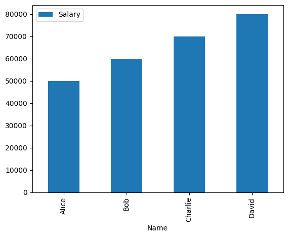
Example: Bar Chart


  import pandas as pd
  import matplotlib.pyplot as plt
  
  # Sample data
  data = {'Name': ['Alice', 'Bob', 'Charlie', 'David'],
          'Age': [25, 30, 35, 40],
          'Salary': [50000, 60000, 70000, 80000]}
  df = pd.DataFrame(data)
  
  # Plotting a bar chart
  df.plot(kind='bar', x='Name', y='Salary')
  plt.show()

Output:

Visualizing Data with Pandas and Matplotlib/Seaborn

Introduction to Data Visualization

Data visualization is a crucial aspect of data analysis, allowing you to represent data graphically to uncover patterns, trends, and insights. Effective visualizations can make complex data more accessible and understandable.

Plotting with Matplotlib for Pandas Data

Matplotlib is a comprehensive library for creating static, animated, and interactive visualizations in Python. It integrates seamlessly with Pandas, making it easy to plot data directly from DataFrames.

Example: Basic Plotting with Matplotlib


  import pandas as pd
  import matplotlib.pyplot as plt
  
  # Sample data
  data = {'Name': ['Alice', 'Bob', 'Charlie', 'David'],
          'Age': [25, 30, 35, 40]}
  df = pd.DataFrame(data)
  
  # Plotting a bar chart
  df.plot(kind='bar', x='Name', y='Age')
  plt.title('Age of Individuals')
  plt.xlabel('Name')
  plt.ylabel('Age')
  plt.show()

Output:

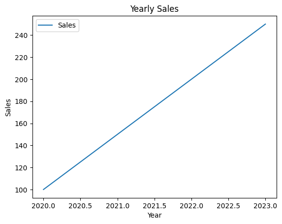
Example: Line Plot


  import pandas as pd
  import matplotlib.pyplot as plt
  
  # Sample data
  data = {'Year': [2020, 2021, 2022, 2023],
          'Sales': [100, 150, 200, 250]}
  df = pd.DataFrame(data)
  
  # Plotting a line chart
  df.plot(kind='line', x='Year', y='Sales')
  plt.title('Yearly Sales')
  plt.xlabel('Year')
  plt.ylabel('Sales')
  plt.show()

Output:

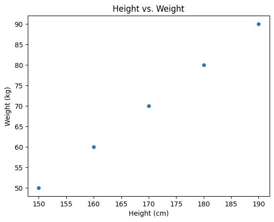
Advanced Visualization with Seaborn

Seaborn is built on top of Matplotlib and provides a high-level interface for drawing attractive and informative statistical graphics. It is particularly useful for visualizing complex datasets.

Example: Scatter Plot with Seaborn


  import pandas as pd
  import seaborn as sns
  import matplotlib.pyplot as plt
  
  # Sample data
  data = {'Height': [150, 160, 170, 180, 190],
          'Weight': [50, 60, 70, 80, 90]}
  df = pd.DataFrame(data)
  
  # Plotting a scatter plot
  sns.scatterplot(data=df, x='Height', y='Weight')
  plt.title('Height vs. Weight')
  plt.xlabel('Height (cm)')
  plt.ylabel('Weight (kg)')
  plt.show()

Output:

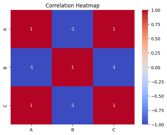
Example: Heatmap with Seaborn


  import pandas as pd
  import seaborn as sns
  import matplotlib.pyplot as plt
  
  # Sample data
  data = {'A': [1, 2, 3, 4],
          'B': [4, 3, 2, 1],
          'C': [5, 6, 7, 8]}
  df = pd.DataFrame(data)
  
  # Plotting a heatmap
  sns.heatmap(df.corr(), annot=True, cmap='coolwarm')
  plt.title('Correlation Heatmap')
  plt.show()

Output:

Additional Examples

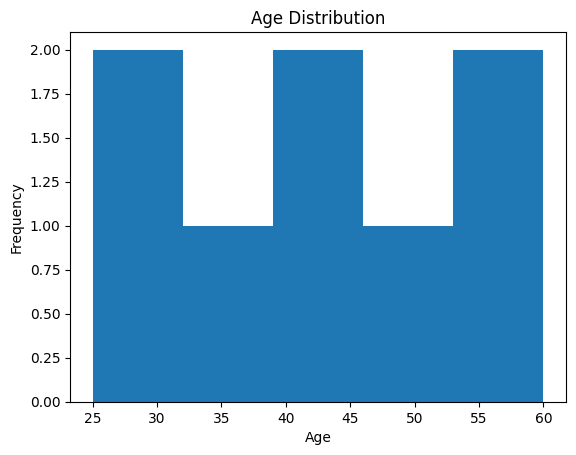
Histogram with Matplotlib

Histograms are useful for visualizing the distribution of a dataset.


  import pandas as pd
  import matplotlib.pyplot as plt
  
  # Sample data
  data = {'Age': [25, 30, 35, 40, 45, 50, 55, 60]}
  df = pd.DataFrame(data)
  
  # Plotting a histogram
  df['Age'].plot(kind='hist', bins=5)
  plt.title('Age Distribution')
  plt.xlabel('Age')
  plt.ylabel('Frequency')
  plt.show()

Output:

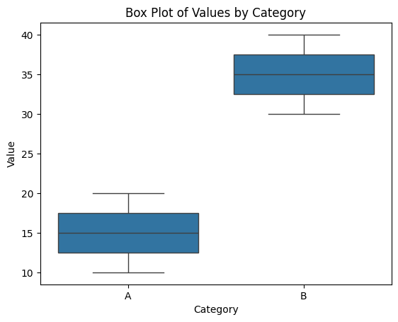
Box Plot with Seaborn

Box plots are useful for visualizing the distribution and identifying outliers.


  import pandas as pd
  import seaborn as sns
  import matplotlib.pyplot as plt
  
  # Sample data
  data = {'Category': ['A', 'A', 'B', 'B'],
          'Value': [10, 20, 30, 40]}
  df = pd.DataFrame(data)
  
  # Plotting a box plot
  sns.boxplot(data=df, x='Category', y='Value')
  plt.title('Box Plot of Values by Category')
  plt.xlabel('Category')
  plt.ylabel('Value')
  plt.show()

Output:

Case Study: End-to-End Data Analysis with Pandas

Problem Statement

In this case study, we aim to analyze sales data to understand trends and patterns. Our goal is to identify the best-selling products, peak sales periods, and customer demographics that contribute most to sales.

Data Import to Insight Generation

Step 1: Importing Data

First, we need to import the sales data from a CSV file into a Pandas DataFrame.


  import pandas as pd
  
  # Importing the sales data
  df = pd.read_csv('sales_data.csv')
  print(df.head())

Step 2: Data Cleaning

Next, we clean the data by handling missing values, correcting data types, and removing duplicates.


  # Handling missing values
  df.dropna(inplace=True)
  
  # Correcting data types
  df['Date'] = pd.to_datetime(df['Date'])
  
  # Removing duplicates
  df.drop_duplicates(inplace=True)

Step 3: Data Transformation

We transform the data to make it suitable for analysis. This includes creating new columns, aggregating data, and normalizing values.


  # Creating a new column for total sales
  df['Total_Sales'] = df['Quantity'] * df['Price']
  
  # Aggregating data by product
  product_sales = df.groupby('Product')['Total_Sales'].sum().reset_index()

Step 4: Insight Generation

We generate insights by performing various analyses, such as identifying the best-selling products and peak sales periods.


  # Identifying best-selling products
  best_selling_products = product_sales.sort_values(by='Total_Sales', ascending=False)
  print(best_selling_products.head())
  
  # Identifying peak sales periods
  df['Month'] = df['Date'].dt.month
  monthly_sales = df.groupby('Month')['Total_Sales'].sum().reset_index()
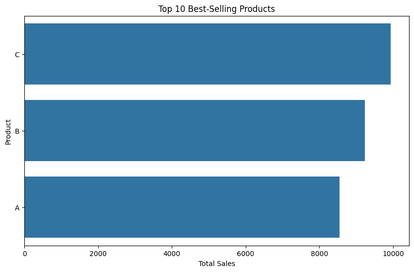
  print(monthly_sales)

Visualization and Reporting

Step 5: Visualizing Data

We use Matplotlib and Seaborn to create visualizations that help us understand the data better.


  import matplotlib.pyplot as plt
  import seaborn as sns
  
  # Plotting best-selling products
  plt.figure(figsize=(10, 6))
  sns.barplot(data=best_selling_products.head(10), x='Total_Sales', y='Product')
  plt.title('Top 10 Best-Selling Products')
  plt.xlabel('Total Sales')
  plt.ylabel('Product')
  plt.show()
  
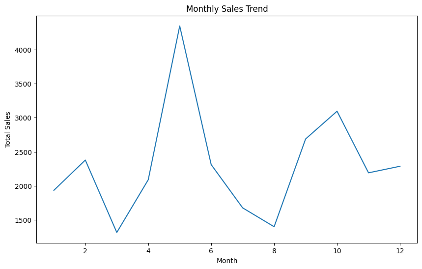
  # Plotting monthly sales
  plt.figure(figsize=(10, 6))
  sns.lineplot(data=monthly_sales, x='Month', y='Total_Sales')
  plt.title('Monthly Sales Trend')
  plt.xlabel('Month')
  plt.ylabel('Total Sales')
  plt.show()

Output:

Step 6: Reporting

Finally, we compile our findings into a report, summarizing the key insights and visualizations.

Sales Data Analysis Report

Key Insights

Top 10 Best-Selling Products: Product A, Product B, Product C, etc.
Peak Sales Periods: Highest sales observed in months X, Y, and Z.

Visualizations

Bar Chart: Top 10 Best-Selling Products
Line Chart: Monthly Sales Trend

Recommendations

Focus marketing efforts on best-selling products.
Plan inventory and staffing around peak sales periods.

Additional Information

Advanced Analysis

Customer Demographics: Analyze customer data to understand which demographics contribute most to sales.
Sales Forecasting: Use time series analysis to forecast future sales trends.

Real-World Examples Across Industries

Finance: Analyzing Stock Market Trends with Pandas

Discover how a financial analyst uses Pandas to analyze stock market trends, predict future prices, and inform investment decisions.


        # Example: Analyzing stock prices
        import pandas as pd
        import yfinance as yf
        
        # Download stock data
        data = yf.download('AAPL', start='2020-01-01', end='2022-02-26')
        
        # Calculate daily returns
        data['Return'] = data['Close'].pct_change()
        
        # Plot the returns
        import matplotlib.pyplot as plt
        data['Return'].plot(figsize=(10,6))
        plt.title('Daily Returns of AAPL')
        plt.xlabel('Date')
        plt.ylabel('Return')
        plt.show()

Healthcare: Patient Outcome Analysis with Pandas

Learn how healthcare professionals utilize Pandas to analyze patient outcomes, identifying key factors influencing recovery rates and informing treatment plans.


        # Example: Analyzing patient outcomes
        import pandas as pd
        
        # Sample patient data
        data = {'Patient_ID': [1, 2, 3],
                'Treatment': ['A', 'B', 'A'],
                'Outcome': ['Recovered', 'Not Recovered', 'Recovered']}
        df = pd.DataFrame(data)
        
        # Analyze recovery rates by treatment
        outcome_rates = df['Treatment'].value_counts(normalize=True)
        print(outcome_rates)

Environmental Science: Climate Data Analysis with Pandas

Explore how environmental scientists leverage Pandas to analyze climate data, understanding global temperature trends and the impact of human activities.


        # Example: Analyzing global temperatures
        import pandas as pd
        
        # Sample climate data
        data = {'Year': [2000, 2001, 2002],
                'Temperature': [15.2, 15.5, 15.8]}
        df = pd.DataFrame(data)
        
        # Plot temperature trends
        import matplotlib.pyplot as plt
        df.plot(x='Year', y='Temperature', figsize=(10,6))
        plt.title('Global Temperature Trend')
        plt.xlabel('Year')
        plt.ylabel('Temperature (°C)')
        plt.show()

Advanced Topics and Best Practices

Optimizing Pandas for Performance: Tips and Tricks

1. Use Vectorized Operations

Vectorized operations in Pandas are designed to perform computations more efficiently by applying operations to entire arrays rather than individual elements. This can significantly speed up your data processing tasks.

Example: Vectorized Operations


  import pandas as pd
  
  # Sample data
  data = {'A': [1, 2, 3, 4, 5]}
  df = pd.DataFrame(data)
  
  # Vectorized operation to square each element
  df['A_squared'] = df['A'] ** 2
  print(df)

2. Efficient Data Storage with Categoricals

Using categorical data types can reduce memory usage and improve performance, especially when dealing with columns that have a limited number of unique values.

Example: Using Categoricals


  import pandas as pd
  
  # Sample data
  data = {'City': ['New York', 'Los Angeles', 'Chicago', 'New York', 'Chicago']}
  df = pd.DataFrame(data)
  
  # Converting to categorical data type
  df['City'] = df['City'].astype('category')
  print(df.info())

3. Leveraging Dask for Large Datasets

Dask is a parallel computing library that scales Pandas workflows to larger-than-memory datasets. It allows you to work with large datasets by breaking them into smaller, manageable chunks and processing them in parallel.

Example: Using Dask with Pandas


  import dask.dataframe as dd
  
  # Reading a large CSV file with Dask
  df = dd.read_csv('large_data.csv')
  
  # Performing operations on the Dask DataFrame
  result = df.groupby('column_name').mean().compute()
  print(result)

Additional Tips for Optimizing Pandas Performance

4. Use apply() Sparingly

While apply() is a powerful function, it can be slower than vectorized operations. Use it only when necessary.

Example: Using apply() Sparingly

# Example of using apply() sparingly
  df['A_squared'] = df['A'].apply(lambda x: x ** 2)

5. Optimize Memory Usage

Monitor and optimize memory usage by using appropriate data types and avoiding unnecessary copies of DataFrames.

Example: Optimizing Memory Usage


  # Example of optimizing memory usage
  df['A'] = df['A'].astype('int32')

6. Use Chunking for Large Files

When dealing with large files, read them in chunks to avoid memory overload.

Example: Reading a Large File in Chunks


  # Example of reading a large file in chunks
  chunk_size = 10000
  chunks = pd.read_csv('large_data.csv', chunksize=chunk_size)
  for chunk in chunks:
      process(chunk)

Future of Pandas and Emerging Trends in Data Science

Upcoming Features and Releases

Pandas continues to evolve with new features and improvements aimed at enhancing performance and usability. Some of the upcoming features include:

Enhanced Performance: Ongoing efforts to optimize performance, especially for large datasets, through better memory management and faster computation.
Improved Integration with Other Libraries: Enhancements to ensure seamless integration with other data science libraries like Dask, NumPy, and Scikit-learn.
New Data Manipulation Functions: Introduction of new functions to simplify complex data manipulation tasks, making it easier for users to handle and analyze data.